


The True Power of ROUNDing in Excel
An overview of all rounding functions in Excel with practical examples on how to leverage them in your daily work.

If you’ve ever seen a financial report, even for a brief moment, you know they usually present values in thousands. And that makes a lot of sense. It allows us not to worry about minor discrepancies when preparing financial statements and other reports. It also makes the amounts easier to read.
However, this can be very misleading in your day-to-day work, especially if you spend time looking at various reports, and from various entities. Many internal reports are not prepared in thousands, as they need to be more precise. So, the occasional summary report might slip through and baffle you for a few minutes until you figure out it’s presented in thousands.
I am 101% sure this seems like such a nitpicky problem, but I assure you, it’s not. So, trust me and read on.

A few years back, I was working with a consultant and noticed something pretty great. They showed everything in thousands with 3 trailing zeros. So, instead of presenting $34,560.25 as $35 thousand, they presented it as $35,000. I’ve always felt that showing numbers in thousands diminished their true weight and impact, which is quite important in a financial setting. But here was some 4-tier audit consultant who had cracked it.
$35,000 is so much easier to read than $34,560.25 and, at the same time, it carries so much more weight than $35k.
Okay, feel free to laugh at me for being so excited about presentation of financial data, but I bet you didn’t know you can present numbers like this with the ROUND function in Excel!
So, the ROUND function takes 2 parameters:
Value to be rounded;
Number of digits after the decimal point to round to.
Did you know the second one can have a negative value? Say what!
Here’s a table showing a regular ROUND usage, a presentation in thousands, and the ROUND function with number of digits after the decimal point equal to -3:

I don’t know about you, but I have strong preferences towards the latter presentation method. It makes everything so much clearer.
Of course, this is not all ROUND can do. There are two more rounding functions in Excel – ROUNDUP and ROUNDDOWN, and they have some pretty useful applications in real life.
Here’s a real-life example of using ROUNDUP. When I was working in a high turnover manufacturing plant, I constantly had to forecast new FTEs (full-time employees) and associated costs with recruiting, hiring, etc.
My calculations got complex with time and never resulted in whole numbers. For example, I will consider production capacities, demand, etc., and end up with 12.3 FTEs needed. However, you cannot hire 0.3 of a person, so you need to calculate with 13 to be correct. I ignored this up until at some point I decided to use ROUNDUP to round all numbers of FTEs upwards. The total change in costs across my entire workforce model was $75,000. Quite the rounding error.
Here's an example of using ROUNDUP to round FTE numbers upwards, with zero digits after the decimal point.
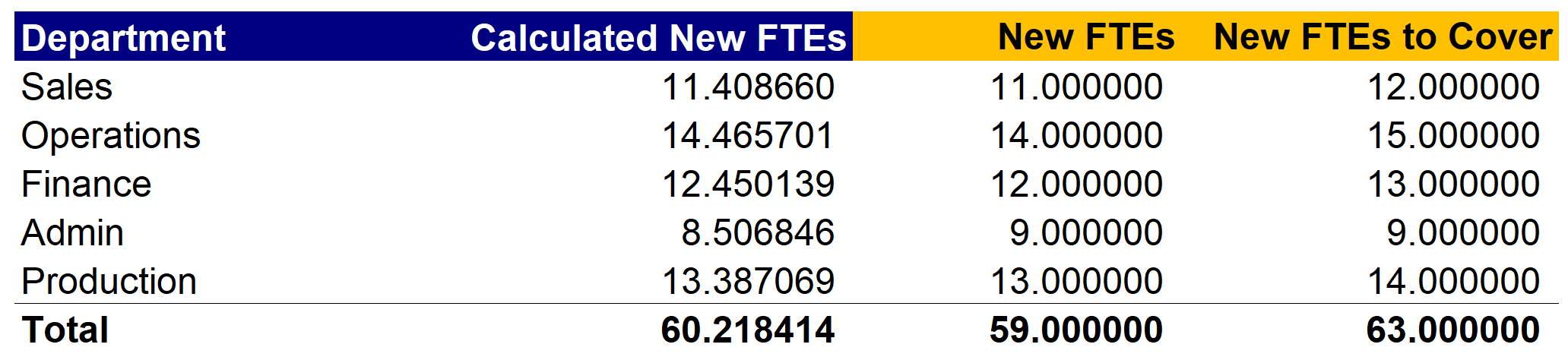
Notice that if we use the regular ROUND function, we end up with 59 people who don’t cover our needs. On the other hand, if we use ROUNDUP, we can see that we actually need almost 3 more employees in total. This is because we must round up per department, and not as a total. Now imagine we have to budget $5k of recruiting fee per employee, and you see we are already $15k short in our budget just because of this rounding thingy. Powerful stuff!
Here's another practical example, for ROUNDDOWN this time. You are an IT manager and need to distribute your team’s roaming data plan to the team members. Your plan grants you 13,000 GB of traffic abroad. Including yourself, the team has 7 members. You decide to divide it equally and end up at 1,857.14 GB per member. However, the provider works with 1 GB as the lowest step. You can use ROUNDDOWN to make sure you are not exceeding your total, and you are also presenting in a way that works for everyone.
Below is an example of using ROUNDDOWN for this exact scenario.

In the first calculation we use ROUNDDOWN to ensure that we end up with the lower whole number, thus never exceeding the available total. Now imagine that the step was 100 GB. We can then use -2 as the number of digits after the decimal point when writing our ROUNDDOWN function. This is how you get the second calculation. It doesn’t use all the available data, but it meets the requirements.
By now, you should be pretty excited about the ROUND family of functions in Excel. Although, let’s be honest, you probably loved those guys already. I love them so much, that I even built an entire tool within my Excel add-in that allows you to wrap cells in rounding functions in bulk.
Here’s the tool in action:

And here’s the result rounding to -3 digits after the decimal point:

Pretty cool, right?
This is one of my favorite features in the add-in, and one that I use a lot. You can check out all the 30+ time-saving features of Minty Tools for Excel here. And, since you made it this far, here’s a 50% discount code if you decide to give it a go. Just use the promo code MINTY50S during checkout to get 50% off.
Okay, that’s all I wanted to share today (plus plug in my Excel add-in).
Thanks for reading and for sharing with a friend or two, that is the best way to support me (apart from buying the add-in) and help me grow the newsletter and reach more people who might find what I have to share interesting.
See you next week!
Best,
Dobri 🍃